The Hard Side of Noise Reduction - Hardware Based Approach via Beamforming

Speech and noise

From an important conversation with a friend to a professional presentation, speech is essential to human nature. Above all else, it’s how we communicate. So it’s hard to overstate the importance of communicating in a clear and effective way.

One of the most critical aspects of effective communication is speech comprehensibility. To assess it, we use a well-known measure called speech intelligibility. Some factors that can harm intelligibility include background noise, other people talking near the speaker, and reverberation, also called room echo. Studies show that a decline in communication efficiency due to background noise and reverberation can be substantial (see for example [6] and [8], also [7] for an overview of speech communication).

Being a problem of paramount importance, myriad works are devoted to enhancing the quality of speech recorded in noisy conditions. The solutions and approaches to this problem can be roughly partitioned into two categories: software-based and hardware-based, without precluding the combination of both.

It all starts with hardware when we use a microphone to record a sound. However, under typical environmental conditions, a single microphone may perform poorly in capturing the sound of interest (e.g. the speaker’s voice) because the microphone will also pick up nearby sounds, adversely affecting speech intelligibility. To address this problem, many consumer electronic devices, such as laptops, smartphones, tablets, and headsets, may use multiple microphones to capture the same audio stream (see [1] and [2] for practical examples).

Interfering Waves

To show how several microphones might become helpful for voice enhancement, we need to understand the physics that govern sound. In its basic definition, sound is a vibration propagating through a transmission medium (e.g. air or water) as an acoustic wave. The principle of superposition states that in linear systems the net response at a given point of several stimuli is the sum of the responses of each stimulus as if they were acting separately. This principle applied to sound signals coming from several sources implies (under linear time invariance of a microphone) that the net effect recorded by a microphone will be the sum of individual sources. Essentially, this means that sound waves can combine to either amplify or reduce each other.

An interesting observation here is that, depending on the microphone’s position, the signal from some of the sources might be reduced (attenuated). Just think about two stones dropped into a pond: the two waves that are formed will add to create a wave of greater or lower amplitude, depending on where in the pond we look. This phenomenon, when two or more waves are combined, is called wave interference. We then distinguish between constructive and destructive interference, depending on whether the amplitude of the combined wave is larger or smaller than the constituent waves.

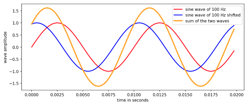
Figure 1. The orange-colored curve is the sum (the result of interference) of two sine waves of 100 Hz where one of the waves is slightly shifted in time. Observe that the amplitude of the combined wave is smaller than the sum of the amplitudes of the individual waves.

A common application of wave interference is active noise cancellation (ANC) in headsets. Here, a signal of the same amplitude as the captured noise but with an inverted phase is emitted by a noise-canceling speaker to reduce the unwanted noise. The interference between the original signal (the noise) and the generated one (with anti-phase) is destructive, resulting in noise reduction.

Enter Beamforming

By leveraging wave interference, one may then try to use several microphones to reinforce the signal coming from the direction of the main speaker (constructive interference) while suppressing signals from other directions (destructive interference). This is what beamforming does.

Audio beamforming, also known as spatial filtering, is a commonly used method for noise reduction. In a nutshell, it is a digital signal processing (DSP) technique that processes and combines sound received by a microphone array (see Figure 2) to enable the preferential capture of sound coming from specific directions. In other words, depending on which direction the microphone receives the sound from, the signal will experience constructive or destructive interference with its time-shifted replicas (see Figure 1).

The Delay and Sum Beamforming Technique

There are many beamforming algorithms. For the exposition, we will concentrate on the most basic form of it, which despite its simplicity, conveys the main ideas at the heart of the method.

Assume we have a linear uniform array of microphones, i.e. all of the microphones are arranged in a straight line with an equal distance between each other. For a source located sufficiently far from the array, we can model a sound emitting from it and reaching the microphones as a planar wave. Indeed, the sound waves propagate in spherical fronts, and the sphere’s curvature decreases as its radius extends. Thanks to this and the assumption of a distant source, we get an almost flat surface near the receiver (see Figure 2).

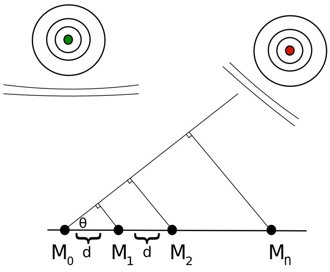
Figure 2. This schematic view represents a linear microphone array, where M-s stand for microphones, and d is the distance between them. The signal source, indicated in green, is located perpendicular (at 90 degrees) to the microphone array, where for the reference point on the array we take the leftmost microphone M0. The noise source, depicted in red, is seen from the array at a different angle denoted by θ. Observe that the source will reach all microphones simultaneously, while the noise arrives at the rightmost microphone first before getting to the rest in the array.

Recall that beamforming aims to capture signals from specific preferential directions and suppress signals from other directions. Let’s assume that the preferential direction is perpendicular to the microphone array. We will see later that this results in no loss of generality.

Since we assumed that the audio source is located far away from the microphone array, we can say that the waves traveling from the source to individual microphones are almost parallel, just as lines from either Los Angeles or San Diego to New York would likewise be virtually parallel. This implies that the angle between these rays and the line on which the array is positioned does not change from microphone to microphone.

Next, depending on the position of the source, the sound waves emitting from it might reach the microphones at different times. This means that while each microphone in the array records the same signal, they will be slightly shifted in time. Taking the leftmost microphone on the array as our reference, we can easily calculate the time delays with respect to the reference microphone, by using our assumption of parallel rays and relying on the fact that the speed of sound in air is constant. We then sum the reference signal (the one recorded by the leftmost microphone) with its time-shift replicas and divide the sum by the number of microphones in the array to normalize the net signal. Depending on the size of the delays and wavelength of the signal, we can get destructive interference. Note that for our direction of interest, which was fixed at 90 degrees (see Figure 2), there is no time shift in the captured signals; hence the same summing followed by the normalization procedure results in the reference signal recorded at the leftmost microphone.

The process just described is called delay and sum beamforming, and it is the simplest form of beamforming method. Our assumption of the source is at 90 degrees can be replaced by any angle. Indeed, for a given angle we can compute the expected delays described above and apply the delay corresponding to a given microphone on a signal recorded by it. This will align the signals as if they arrived simultaneously, similar to the perpendicular case. This procedure of adjusting the directionality of the array is called steering.

The microphone array’s topology also directly affects the result of the delay and sum method. To illustrate how the delay and sum algorithm works, we perform a numerical simulation for 20 microphones with an inter-microphone distance of 0.08 meters, where the input signal is a sine wave of 1000 Hz. The images below show how the array responds to this source, depending on the direction of arrival. We transform the amplitude of the resulting wave to decibel scale (dB), referring to it as the gain of the array.

array of 20 microphones placed

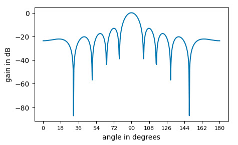
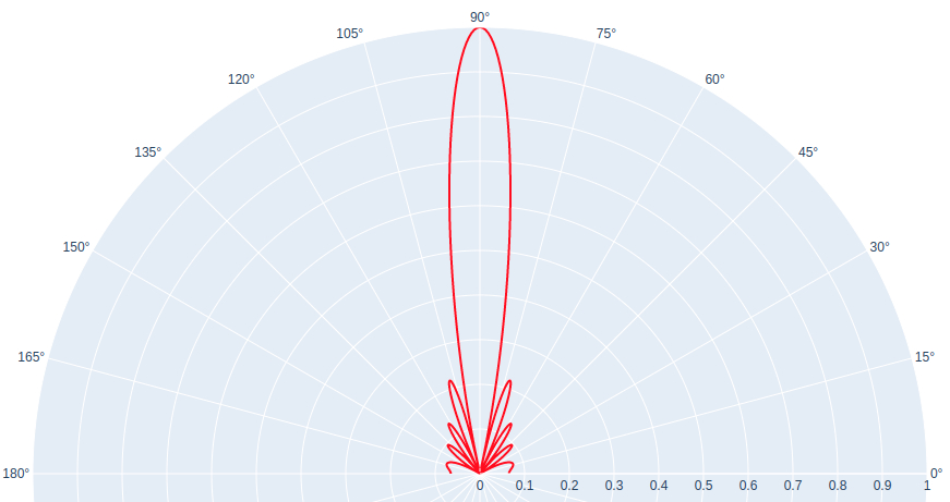
Figure 3. The first image shows the gain of an array of 20 microphones placed 0.08 meters away from each other on a sine wave of 1000 Hz for angles in the range of 0 to 180. Notice that we have a peak at 90 degrees, while the rest of the angles experience attenuation. The second image depicts the same graph as above in polar coordinates, with the original amplitudes without passing to a dB scale. Here we see a beam forming at 90 degrees (cf. beamforming), and smaller beams at other degrees.

The gain of the array varies with frequency. The graphs below show gains of frequencies ranging from 0 to 8000 Hz for arrays of 10, 20, and 40 microphones respectively, arranged in a line with 0.08 meters of inter-microphone distance. Remarkably, the array cannot suppress specific signals of high frequencies, although the arrival angle differs from the preferred one. This phenomenon, called spatial aliasing, happens when a linear array detects signals whose wavelengths are not long enough compared to the distance between array elements.

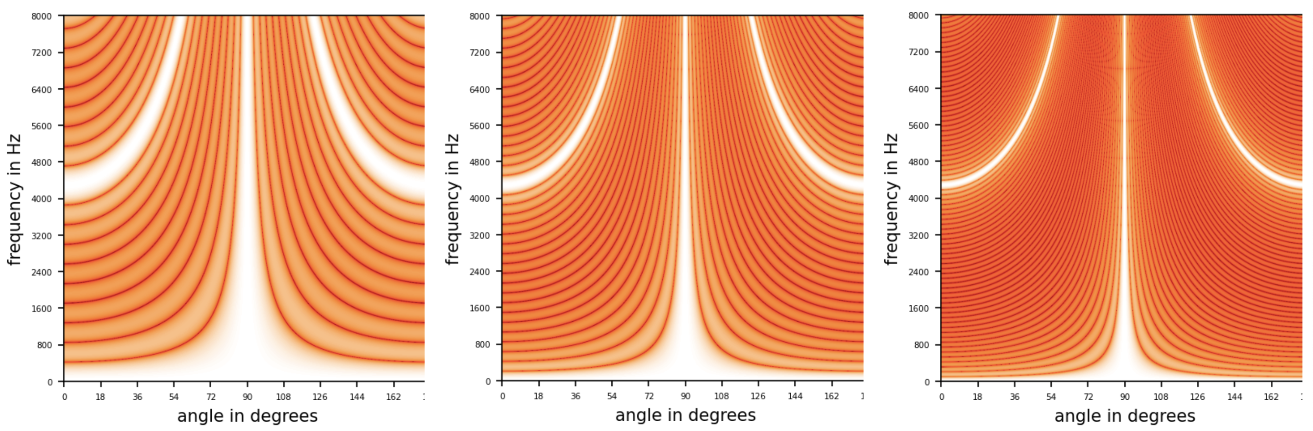
Figure 4. The gain of a source signal for frequencies ranging from 0 to 8000 Hz for a linear array of microphones with 10, 20, 40 elements respectively, with 0.08 meter distance between microphones. The lighter the color, the more significant the gain, while darker colors indicate attenuation. Notice that there is a light-coloured sector around 90 degrees. However, there are also lighter sections at other angles for higher frequencies due to spatial aliasing. Observe also that the larger the number of microphones, the stronger the concentration around the preferred direction.

Figure 4. The gain of a source signal for frequencies ranging from 0 to 8000 Hz for a linear array of microphones with 10, 20, and 40 elements respectively, with a 0.08-meter distance between microphones. The lighter the color, the more significant the gain, while darker colors indicate attenuation. Notice that there is a light-colored sector around 90 degrees. However, there are also lighter sections at other angles for higher frequencies due to spatial aliasing. Observe also that the larger the number of microphones, the stronger the concentration around the preferred direction.

Spatial Filtering in Human Auditory System

One of the applications of beamforming technology is sound source localization, which estimates the position of one or many sound sources relative to a given reference point. Remarkably, this happens all the time in our ears.

We’re able to tell where a sound is coming from when we hear it because of a sound localization process that is partially based on binaural cues. More precisely, it’s because of the differences in the arrival time or the intensity of the sounds at the left and right ears. Such differences are used mainly for left-right localization in space.

Beamforming Beyond Sound

Beamforming methods are abundant. Some variations of the method discussed above include amplitude scaling of each signal before the summation stage, setting up microphones in a rather complex arrangement instead of a linear placement, adapting the response of a beamformer automatically (adaptive beamforming), etc.

Beamforming methods also work in the reverse mode, i.e. for signal transmitting instead of receiving. A wide range of applications goes beyond acoustics, as beamforming is employed in radar, sonar, seismology, wireless communications, and more. The interested reader may consult [3], [4], [5], and the references therein for more information.

Audio Enhancement Beyond Beamforming

Although audio beamforming may be effective at reducing noise and increasing speech intelligibility, it relies on specialized hardware. Plus, beamforming alone, does not guarantee the complete elimination of background noises, so the output of spatial filtering usually undergoes further processing before transmission.

At Krisp, we approach the problem of speech enhancement in noisy conditions from a pure software perspective. While we recognize the benefits that spatial filtering can offer, we prioritize the flexibility of deploying and utilizing our solutions on any device, no matter whether it has many microphones or just one.

Try next-level audio and voice technologies

Krisp licenses its SDKs to embed directly into applications and devices. Learn more about Krisp’s SDKs and begin your evaluation today.

References

[1] Dusan, S.V., Paquier, B.P. and Lindahl, A.M., Apple Inc, 2016. System and method of improving voice quality in a wireless headset with untethered earbuds of a mobile device. U.S. Patent 9,532,131.

[2] Iyengar, V. and Dusan, S.V., Apple Inc, 2018. Audio noise estimation and audio noise reduction using multiple microphones. U.S. Patent 9,966,067.

[3] Kellermann, W. (2008). Beamforming for Speech and Audio Signals. In: Havelock, D., Kuwano, S., Vorländer, M. (eds) Handbook of Signal Processing in Acoustics. Springer, New York, NY. https://doi.org/10.1007/978-0-387-30441-0_35

[4] Li, J. and Stoica, P., 2005. Robust adaptive beamforming. John Wiley & Sons.

[5] Liu, W. and Weiss, S., 2010. Wideband beamforming: concepts and techniques. John Wiley & Sons.

[6] Munro, M. (1998). THE EFFECTS OF NOISE ON THE INTELLIGIBILITY OF FOREIGN-ACCENTED SPEECH. Studies in Second Language Acquisition, 20(2), 139-154. doi:10.1017/S0272263198002022 https://www.cambridge.org/core/journals/studies-in-second-language-acquisition/article/abs/effects-of-noise-on-the-intelligibility-of-foreignaccented-speech/67D7F1E4248B019B77DA46825DB70E74#

[7] O’Shaughnessy. Speech communications: Human and machine. 1999.

[8] Puglisi, G.E., Warzybok, A., Astolfi, A. and Kollmeier, B., 2021. Effect of reverberation and noise type on speech intelligibility in real complex acoustic scenarios. Building and Environment, 204, p.108-137.

https://www.sciencedirect.com/science/article/abs/pii/S0360132321005382