Can You Hear a Room?

Introduction

Sound propagation has distinctive features associated with the environment where it happens. Human ears can often clearly distinguish whether a given sound recording was produced in a small room, large room, or outdoors. One can even get a sense of a direction or a distance from the sound source by listening to a recording. These characteristics are defined by the objects around the listener or a recording microphone such as the size and material of walls in a room, furniture, people, etc. Every object has its own sound reflection, absorption, and diffraction properties, and all of them together define the way a sound propagates, reflects, attenuates, and reaches the listener.

In acoustic signal processing, one often needs a way to model the sound field in a room with certain characteristics, in order to reproduce a sound in that specific setting, so to speak. Of course, one could simply go to that room, reproduce the required sound and record it with a microphone. However, in many cases, this is inconvenient or even infeasible.

For example, suppose we want to build a Deep Neural Net (DNN)-based voice assistant in a device with a microphone that receives pre-defined voice commands and performs actions accordingly. We need to make our DNN model robust to various room conditions. To this end, we could arrange many rooms with various conditions, reproduce/record our commands in those rooms, and feed the obtained data to our model. Now, if we decide to add a new command, we would have to do all this work once again. Other examples are Virtual Reality (VR) applications or architectural planning of buildings where we need to model the acoustic environment in places that simply do not exist in reality.

In the case of our voice assistant, it would be beneficial to be able to encode and digitally record the acoustic properties of a room in some way so that we could take any sound recording and “embed” it in the room by using the room “encoding”. This would free us from physically accessing the room every time we need it. In the case of VR or architectural planning applications, the goal then would be to digitally generate a room’s encoding only based on its desired physical dimensions and the materials and objects contained in it.

Thus, we are looking for a way to capture the acoustic properties of a room in a digital record, so that we can reproduce any given audio recording as if it was played in that room. This would be a digital acoustic model of the room representing its geometry, materials, and other things that make us “hear a room” in a certain sense.

What is RIR?

Room impulse response (RIR for short) is something that does capture room acoustics, to a large extent. A room with a given sound source and a receiver can be thought of as a black-box system. Upon receiving on its input a sound signal emitted by the source, the system transforms it and outputs whatever is received at the receiver. The transformation corresponds to the reflections, scattering, diffraction, attenuation and other effects that the signal undergoes before reaching the receiver. Impulse response describes such systems under the assumption of time-invariance and linearity. In the case of RIR, time-invariance means that the room is in a steady state, i.e, the acoustic conditions do not change over time. For example, a room with people moving around, or a room where the outside noise can be heard, is not time invariant since the acoustic conditions change with time. Linearity means that if the input signal is a scaled superposition of two other signals, x and y, then the output signal is a similarly scaled superposition of the output signals corresponding to x and y, individually. Linearity holds with sufficient fidelity in most practical acoustic environments (while time-invariance can be achieved in a controlled environment).

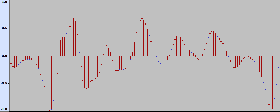
Let us take a digital approximation of a sound signal. It is a sequence of discrete samples, as shown in Fig. 1.

Fig. 1 The waveform of a sound signal.

Each sample is a positive or negative number that corresponds to the degree of instantaneous excitation of the sound source, e.g., a loudspeaker membrane, as measured at discrete time steps. It can be viewed as an extremely short sound, or an impulse. The signal can thus be approximately viewed as a sequence of scaled impulses. Now, given time-invariance and linearity of the system, some mathematics shows that the effect of a room-source-receiver system on an audio signal can be completely described by its effect on a single impulse, which is usually referred to as an impulse response. More concretely, impulse response is a function h(t) of time t > 0 (response to a unit impulse at time t = 0) such that for an input sound signal x(t), the system’s output is given by the convolution between the input and the impulse response. This is a mathematical operation that, informally speaking, produces a weighted sum of the delayed versions of the input signal where weights are defined by the impulse response. This reflects the intuitive fact that the received signal at time t is a combination of delayed and attenuated values of the original signal up to time t, corresponding to reflections from walls and other objects, as well as scattering, attenuation and other acoustic effects.

For example, in the recordings below, one can see the RIR recorded by a clapping sound (see below), an anechoic recording of singing, and their convolution.

RIR

Singing anechoic

Singing with RIR

It is often useful to consider sound signals in the frequency domain, as opposed to the time domain. It is known from Fourier analysis that every well-behaved periodic function can be expressed as a sum (infinite, in general) of scaled sinusoids. The sequence of the (complex) coefficients of sinusoids within the sum, the Fourier coefficients, provides another, yet equivalent representation of the function. In other words, a sound signal can be viewed as a superposition of sinusoidal sound waves or tones of different frequencies, and the Fourier coefficients show the contribution of each frequency in the signal. For finite sequences such as digital audio, that are of practical interest, such decompositions into periodic waves can be efficiently computed via the Fast Fourier Transform (FFT).

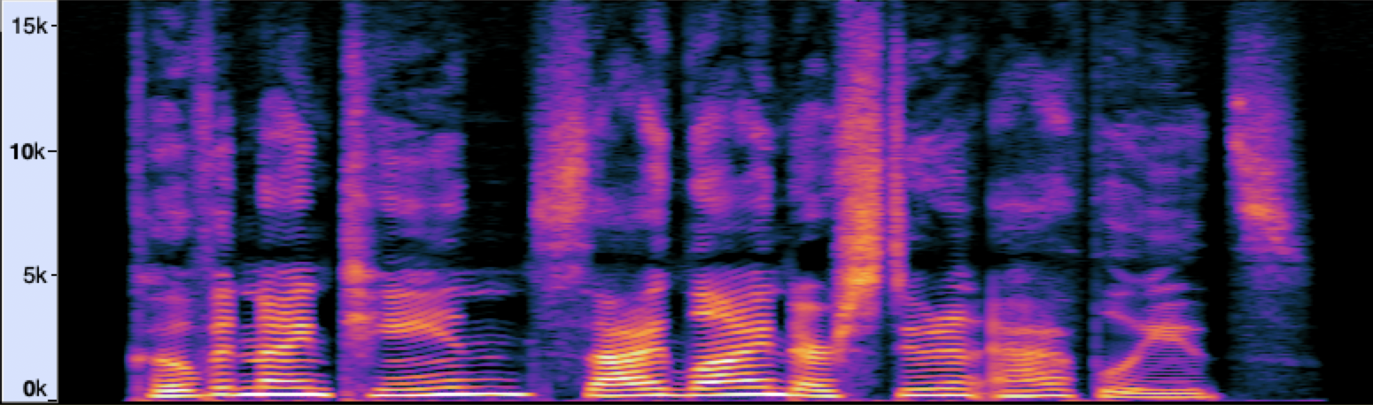
For non-stationary signals such as speech and music, it is more instructive to do analysis using the short-time Fourier transform (STFT). Here, we split the signal into short equal-length segments and compute the Fourier transform for each segment. This shows how the frequency content of the signal evolves with time (see Fig. 2). That is, while the signal waveform and Fourier transform give us only time and only frequency information about the signal (although one being recoverable from another), the STFT provides something in between.

Fig. 2 Spectrogram of a speech signal.

A visual representation of an STFT, such as the one in Fig. 2, is called a spectrogram. The horizontal and vertical axes show time and frequency, respectively, while the color intensity represents the magnitude of the corresponding Fourier coefficient on a logarithmic scale (the brighter the color, the larger is the magnitude of the frequency at the given time).

Measurement and Structure of RIR

In theory, the impulse response of a system can be measured by feeding it a unit impulse and recording whatever comes at the output with a microphone. Still, in practice, we cannot produce an instantaneous and powerful audio signal. Instead, one could record RIR approximately by using short impulsive sounds. One could use a clapping sound, a starter gun, a balloon popping sound, or the sound of an electric spark discharge.

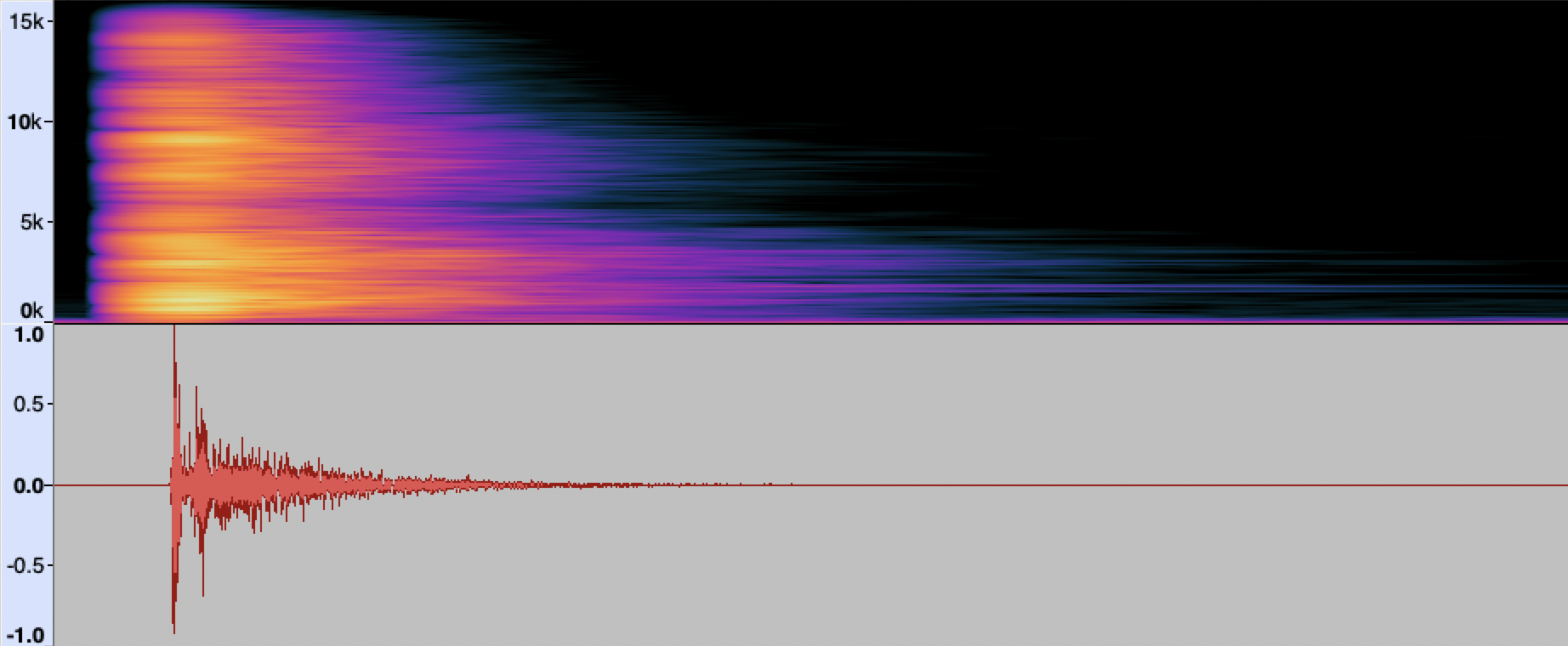
Fig. 3 The spectrogram and waveform of a RIR produced by a clapping sound.

The results of such measurements (see, for example, Fig. 3) may be not sufficiently accurate for a particular application, due to the error introduced by the structure of the input signal. An ideal impulse, in some mathematical sense, has a flat spectrum, that is, it contains all frequencies with equal magnitude. The impulsive sounds above usually significantly deviate from this property. Measurements with such signals may also be poorly reproducible. Alternatively, a digitally created impulsive sound with desired characteristics could be played with a loudspeaker, but the power of the signal would still be limited by speaker characteristics. Among other limitations of measurements with impulsive sounds are: particular sensitivity to external noise (from outside the room), sensitivity to nonlinear effects of the recording microphone or emitting speaker, and the directionality of the sound source.

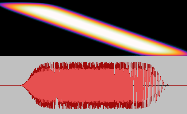
Fortunately, there are more robust methods of measuring room impulse response. The main idea behind these techniques is to play a transformed impulsive sound with a speaker, record the output, and apply an inverse transform to recover impulse response. The rationale is, since we cannot play an impulse as it is with sufficient power, we “spread” its power across time, so to speak, while maintaining the flat spectrum property over a useful range of frequencies. An example of such a “stretched impulse” is shown in Fig. 4.

Fig. 4 A “stretched” impulse.

Other variants of such signals are Maximum Length Sequences and Exponential Sine Sweep. An advantage of measurement with such non-localized and reproducible test signals is that ambient noise and microphone nonlinearities can be effectively averaged out. There are also some technicalities that need to be dealt with. For example, the need for synchronization of emitting and recording ends, ensuring that the test signal covers the whole length of impulse response, and the need for deconvolution, that is applying an inverse transform for recovering the impulse response.

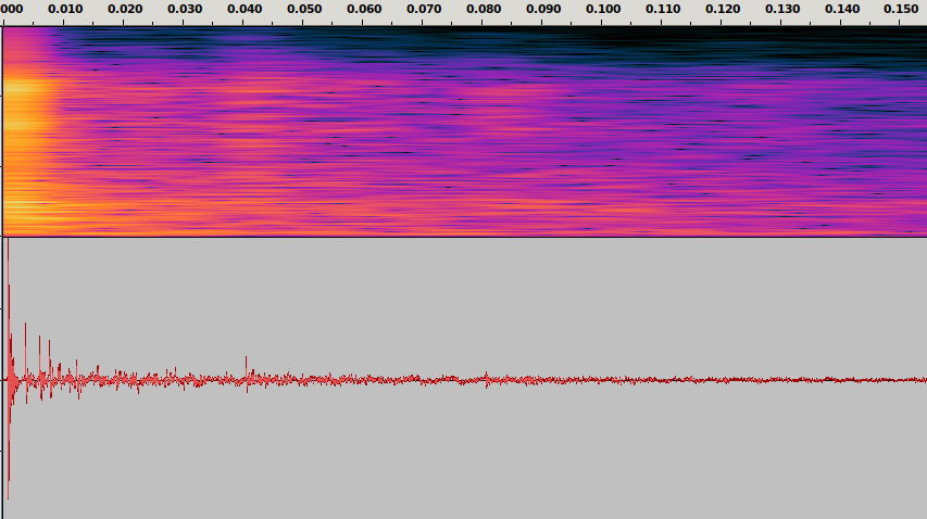
The waveform on Fig. 5 shows another measured RIR. The initial spike at 0-3 ms corresponds to the direct sound that has arrived to the microphone along a direct path. The smaller spikes following it and starting from about 3-5 ms from the first spike clearly show several early specular reflections. After about 80 ms there are no distinctive specular reflections left, and what we see is the late reverberation or the reverberant tail of the RIR.

Fig. 5 A room impulse response. Time is shown in seconds.

While the spectrogram of RIR seems not very insightful apart from the remarks so far, there is some information one can extract from it. It shows, in particular, how the intensity of different frequencies decreases with time due to losses. For example, it is known that intensity loss due to air absorption (attenuation) is stronger for higher frequencies. At low frequencies, the spectrogram may exhibit distinct persistent frequency bands, room modes, that correspond to standing waves in the room. This effect can be seen below a certain frequency threshold depending on the room geometry, the Schroeder frequency, which for most rooms is 20 – 250 Hz. Those modes are visible due to the lower density of resonant frequencies of the room near the bottom of the spectrum, with wavelength comparable to the room dimensions. At higher frequencies, modes overlap more and more and are not distinctly visible.

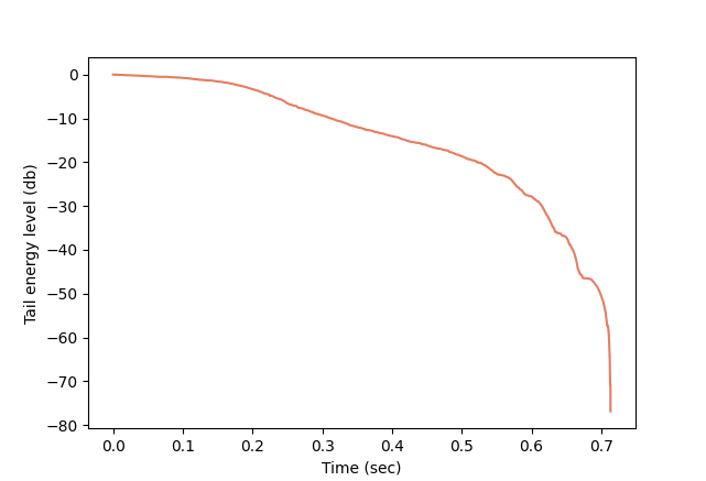
RIR can also be used to estimate certain parameters associated with a room, the most well-known of them being the reverberation time or RT60. When an active sound source in a room is abruptly stopped, it will take longer or shorter time for the sound intensity to drop to a certain level, depending on the room’s geometry, materials, and other factors. In the case of RT60, the question is, how long it takes for the sound energy density to decrease by 60 decibels (dB), that is, to the millionth of its initial value. As noted by Schroeder (see the references), the average signal energy at time t used for computing reverberation time is proportional to the tail energy of the RIR, that is the total energy after time t. Thus, we can compute RT60 by plotting the tail energy level of the RIR on a dB scale (with respect to the total energy). For example, the plot corresponding to the RIR above is shown in Fig. 6:

Fig. 6 The RIR tail energy level curve.

In theory, the RIR tail energy decay should be exponential, that is, linear on a dB scale, but, as can be seen here, it drops irregularly starting at -25 dB. This is due to RIR measurement limitations. In such cases, one restricts the attention to the linear part, normally between the values -5 dB and -25 dB, and obtains RT60 by fitting a line to the measurements of RIR in logarithmic scale, by linear regression, for example.

RIR Simulation

As mentioned in the introduction, one often needs to compute a RIR for a room with given dimensions and material specifications without physically building the room. One way of achieving this would be by actually building a scaled model of the room. Then we could measure the RIR by using test signals with accordingly scaled frequencies, and rescale the recorded RIR frequencies. A more flexible and cheaper way is through computer simulations, by building a digital model of the room and modeling sound propagation. Sound propagation in a room (or other media) is described with differential equations called wave equations. However, the exact solution of these equations is out of reach in most practical settings, and one has to resort to approximate methods for simulations.

While there are many approaches for modeling sound propagation, most common simulation algorithms are based on either geometrical simplification of sound propagation or element-based methods. Element-based methods, such as the Finite Element method, rely on numerical solution of wave equations over a discretized space. For this purpose, the room space is approximated with a discrete grid or a mesh of small volume elements. Accordingly, functions describing the sound field (such as the sound pressure or density) are defined down to the level of a single volume element. The advantage of these methods is that they are more faithful to the wave equations and hence more accurate. However the computational complexity of element-based methods grows rapidly with frequency, as higher frequencies require higher resolution of a mesh (smaller volume element size). For this reason, for wideband applications like speech, element-based methods are often used to model sound propagation only for low frequencies, say, up to 1 kHz.

Geometric methods, on the other hand, work in the time domain. They model sound propagation in terms of sound rays or particles with intensity decreasing with the squared path length from the source. As such, wave-specific interference between rays is abstracted away. Thus rays effectively become sound energy carriers, with the sound energy at a point being computed by the sum of the energies of rays passing through that point. Geometric methods give plausible results for not-too-low frequencies, e.g., above the Schroeder frequency. Below that, wave effects are more prominent (recall the remarks on room modes above), and geometric methods may be inaccurate.

The room geometry is usually modeled with polygons. Walls and other surfaces are assigned absorption coefficients that describe the fraction of incident sound energy that is reflected back into the room by the surface (the rest is “lost” from the simulation perspective). One may also need to model air absorption and sound scattering by rough materials with not too small features as compared to the sound wavelengths.

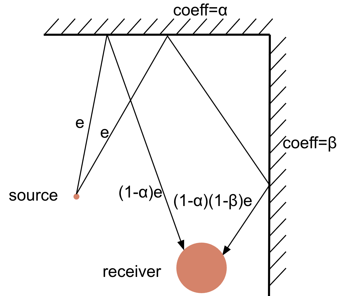
Two well-known geometric methods are stochastic Ray Tracing and Image Source methods. In Ray Tracing, a sound source emits a (large) number of sound rays in random directions, also taking into account directivity of the source. Each ray has some starting energy. It travels with the speed of sound and reflects from the walls while losing energy with each reflection, according to the absorption coefficients of walls, as well as due to air absorption and other losses.

Fig. 7 Ray Tracing (only wall absorption shown).

The reflections are either specular (incident and reflected angles are equal) or scattering happens, the latter usually being modeled by a random reflection direction. The receiver registers the remaining energy, time and angle of arrival of each ray that hits its surface. Time is tracked in discrete intervals. Thus, one gets an energy histogram corresponding to the RIR with a bucket for each time interval. In order to synthesize the temporal structure of the RIR, a random Poisson-distributed sequence of signed unit impulses can be generated, which is then scaled according to the energy histogram obtained from simulation to give a RIR. For psychoacoustic reasons, one may want to treat different frequency bands separately. In this case, the procedure of scaling the random impulse sequence is done for band-passed versions of the sequence, then their sum is taken as the final RIR.

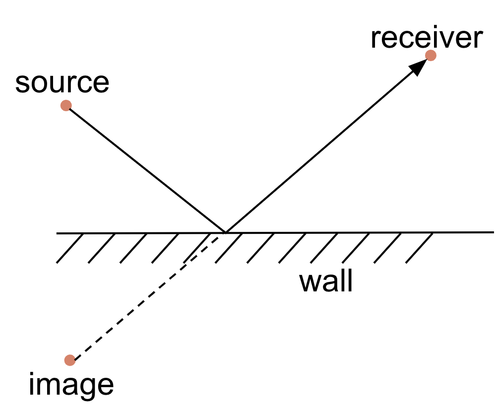
The Image Source method models only specular reflections (no scattering). In this case, a reflected ray from a source towards a receiver can be replaced with rays coming from “mirror images” of the source with respect to the reflecting wall, as shown in Fig. 8.

Fig. 8 The Image Source method.

This way, instead of keeping track of reflections, we construct images of the source relative to each wall and consider straight rays from all sources (including the original one) to the receiver. These first order images cover single reflections. For rays that reach the receiver after two reflections, we construct the images of the first order images, call them second order images, and so on, recursively. For each reflection, we can also incorporate material absorption losses, as well as air absorption. The final RIR is constructed by considering each ray as an impulse that undergoes scaling due to absorption and distance-based energy losses, as well as a distance-based phase shift (delay) for each frequency component. Before that, we need to filter out invalid image sources for which the image-receiver path does not intersect the image reflection wall or is blocked by other walls.

While the Image Source method captures specular reflections, it does not model scattering that is an important aspect of the late reverberant part of a RIR. It does not model wave-based effects either. More generally, each existing method has its advantages and shortcomings. Fortunately, shortcomings of different approaches are often complementary, so it makes sense to use hybrid models that combine several of the methods described above. For modeling late reverberations, stochastic methods like Ray Tracing are more suitable, while they may be too imprecise for modeling the early specular reflections in a RIR. One could further rely on element-based methods like the Finite Element method for modeling RIR below the Schroeder frequency where wave-based effects are more prominent.

Summary

Room impulse response (RIR) plays a key role in modeling acoustic environments. Thus, when developing voice-related algorithms, be it for voice enhancement, automatic speech recognition, or something else, here at Krisp we need to keep in mind that these algorithms must be robust to changes in acoustics settings. This is usually achieved by incorporating the acoustic properties of various room environments, as was briefly discussed here, into the design of the algorithms. This provides our users with a seamless experience, largely independent of the room from which Krisp is being used: they don’t hear the room.